Introduction to Coreset

The Coreset package selects a subset that represents a fixed pool of N items, based on approximate and exact solutions to a suite of objectives:

The Max-Min Diversity Problem (MMDP, the discrete p-dispersion objective) selects $k$ elements such that the minimum distance between any pair of selected elements is as large as possible; the chosen elements are maximally separated. This can reward selections that leave the interior of the set unrepresented. This objective is suited to defining a representative sample from a fixed pool: picking biological specimens for sequencing that span available diversity, or choosing a representative subset of protein structures from a database.

The Max-Sum Diversity Problem (the “maximum diversity problem”) selects $k$ elements that maximize the total pairwise distance they contain. As every pair in the selection contributes to the max-sum score, the optimum tends to favour elements spread across the whole extent of the pool rather than elements that merely avoid a single close neighbour.

The Max-Mean Dispersion Problem maximizes the average distance between selected elements; this differs from the Max Sum objective in that the number of elements to be selected is not specified in advance.

The discrete k-centre problem selects $k$ elements such that the maximum distance from any element in the original set to a selected element is as small as possible. In ensuring that each point has a nearby representative, this objective can select points that reflect a central compromise, rather than selections that are closer to more local points. Whereas dispersion spreads to the extremes, covering gravitates into the interior. This objective is useful when selecting centres that represent each point in a dataset: for example, siting fire stations to guarantee that all buildings can be reached within a given response time.

The maximum-entropy (maxdet) sampling objective selects the $k$ least redundant elements: that is, those that maximize the log-determinant of a similarity kernel built from the distances between them, and thus that together occupy the largest volume.

Installation

Install from CRAN with:

install.packages("Coreset")

Quick start

Our examples employ a built-in R dist object that contains road distances (in km) between 21 European cities.

# Load the `eurodist` dist object
data("eurodist")

# Set a seed for a reproducible selection
set.seed(1)

# Select 4 maximally dispersed cities
ffPick <- FarFirst(4L, eurodist)

# View distances between selected cities
as.matrix(eurodist)[ffPick, ffPick]
#>           Athens Lisbon Stockholm Milan
#> Athens         0   4532      3927  2282
#> Lisbon      4532      0      3231  2250
#> Stockholm   3927   3231         0  2187
#> Milan       2282   2250      2187     0

# Quickly extract the minimum distance for a given selection
MinDist(eurodist, ffPick)
#> [1] 2187

FarFirst() returned the indices of the four cities whose nearest-neighbour distance within the selection is largest. MinDist() reports that value explicitly.

Methods at a glance

Coreset provides solvers for each objective:

Function	Objective	Quality	Speed	Stochastic?
`FarFirst()`	max-min / k-centre	Good (2-approximation)	Very fast	No
`DropAdd()`	MMDP (max-min)	High (≈ 99 % optimal)	Fast	No
`Grasp()`	MMDP (max-min)	Highest	Moderate	Yes (`set.seed()`)
`ExactMaxMin()`	MMDP (max-min)	Optimal (NP-hard)	Slow	No
`ExactMaxSum()`	Max-Sum Diversity	Optimal (NP-hard)	Slow	No
`MaxMean()`	max-mean	High	Time-budgeted	Yes (`set.seed()`)
`KCentre()`	k-centre	Near-optimal	Fast	No
`ExactKCentre()`	k-centre	Optimal (NP-hard)	Slow	No
`MaxEntropy()`	maxdet	High / Optimal for small `k`	Fast	No

To compute the score for an arbitrary selection of points under each objective, use MinDist() (max-min), MeanDist() (max-mean) and KCentreRadius() (k-centre). ExactMaxSum() and MaxEntropy() report their own objective value (total pairwise distance and log-determinant respectively) as the score attribute of the selection they return.

Fast greedy selection

The González (1985) algorithm builds the selection greedily: start from a seed point, then repeatedly add whichever unselected point is farthest from the current selection. This greedy rule guarantees a 2-approximation to the optimal T_k and runs in O(N · m) time.

The choice of seed point influences the quality of the selection. Peripheral seeds are more likely than central seeds to represent extremes of the data, and hence to feature in the optimal selection. FarFirst() supports several methods for identifying starting points for the greedy search.

The default is a two-step strategy that starts from a random selects a point at random, then starts greedy search from the point furthest from

By default FarFirst() runs three "random_furthest" starts, each of which takes a randomly selected point, moves to the point furthest from it, and begins the farthest-first sweep from there. The results of the pass with the highest T_k are returned. Three starts captures most of the quality gain from restarting — on benchmarks across a wide range of datasets the improvement curve bends early (knee at n ≈ 3–4); for higher-quality results, prefer DropAdd(), whose tabu search escapes the plateau that restarts cannot.

set.seed(1)
FarFirst(6L, eurodist)   # default: best of three random starts
#> 6 elements (1 12 20 16 5 2) selected by farthest-first (best of 3 strategies, 3 tied: random_furthest1, random_furthest2, random_furthest3), each at distance >= 1014

The number of random starts can be configured via the nSeeds argument.

set.seed(1)
# Fewer starts provides a faster run, but the solution found may be inferior
FarFirst(6L, eurodist, nSeeds = 2L)
#> 6 elements (1 12 20 16 5 2) selected by farthest-first (best of 2 strategies, 2 tied: random_furthest1, random_furthest2), each at distance >= 1014

Other strategies to select peripheral seeds are available via the strategy argument; these are described at PickPoint(). The best solution from the requested strategies is used.

ffPick <- FarFirst(6L, eurodist, strategy = c("diameter", "anti_medoid"))
MinDist(eurodist, ffPick)
#> [1] 1014

attr(ffPick, "winning_strategy")
#> [1] "diameter"    "anti_medoid"

With large datasets of points that are not associated with natural coordinates, it may not be feasible to compute and store all N×N distances. In such cases, a distance function may take the place of the distance matrix. This function is passed one index i at a time, and must return the distance from i to each other point. N, the number of objects, must also be specified.

data("USArrests")
arrestTypes <- USArrests[, c("Murder", "Assault", "Rape")]
StateDist <- function(i) {
  diffs <- sweep(arrestTypes, 2, unlist(arrestTypes[i, ]), "-")
  sqrt(rowSums(diffs ^ 2))
}
idx <- FarFirst(4L, StateDist, N = nrow(arrestTypes), strategy = 1L)
arrestTypes[idx, ]
#>                Murder Assault Rape
#> Alabama          13.2     236 21.2
#> North Dakota      0.8      45  7.3
#> North Carolina   13.0     337 16.1
#> Washington        4.0     145 26.2

DropAdd tabu search

The DropAdd heuristic (Porumbel et al., 2011) refines an initial selection by alternately dropping and adding points from the selection; it typically reaches ≈ 99 % of the optimal T_k.

daPick <- DropAdd(6L, eurodist, plateau = 500L)

daPick
#> 6 elements (1 2 5 12 20 21) selected by DropAdd tabu search, each at distance >= 1294
labels(eurodist)[daPick]
#> [1] "Athens"    "Barcelona" "Cherbourg" "Lisbon"    "Stockholm" "Vienna"

The algorithm terminates after plateau iterations do not improve T_k. Where N is too large for a distance matrix to fit in memory (roughly N > 46 000), pass a coordinate matrix via DropAdd(points = ...).

GRASP with path relinking

GRASP + path relinking (Resende et al., 2010) combines a randomised greedy construction phase with extended local search, and then refines an “elite” set of good solutions by interpolating between elite-pair trajectories (path relinking). It achieves the highest T_k of the three heuristics, at a proportionally higher cost.

set.seed(0)
grPick <- Grasp(6L, eurodist, plateau = 50L)
grPick
#> 6 elements (1 2 4 12 20 21) selected by GRASP with path-relinking, each at distance >= 1305
labels(eurodist)[grPick]
#> [1] "Athens"    "Barcelona" "Calais"    "Lisbon"    "Stockholm" "Vienna"
attr(grPick, "pr_calls")   # path-relinking calls performed
#> [1] 90

plateau controls how many consecutive non-improving GRASP iterations trigger termination; maxSeconds is available as an absolute time cap.

Comparing methods on a simulated example

To see how the methods relate visually, we generate 50 points in two dimensions and select k = 8 from each.

set.seed(1) # Seed selected such that FarFirst < DropAdd < Grasp
pts <- matrix(rnorm(100), ncol = 2)   # 50 points, 2 dimensions
d50 <- dist(pts)
k   <- 8L

set.seed(1) # Seed selected such that FarFirst < DropAdd < Grasp
ffPick <- FarFirst(k, d50)
da50Pick <- DropAdd(k, d50, plateau = 500L)
gr50Pick <- Grasp(k, d50, plateau = 50L)

Even a small difference in T_k can correspond to a meaningfully more dispersed selection.

scores <- c(
  FarFirst  = attr(ffPick, "score"),
  DropAdd = attr(da50Pick, "score"),
  Grasp   = attr(gr50Pick, "score")
)
round(scores, 3)
#> FarFirst  DropAdd    Grasp 
#>    1.271    1.369    1.485

Plotting the selections against the point cloud makes the differences concrete. When two methods select the same index, their symbols overlap; the T_k table above captures the quality distinction even when the visual overlap is high.

methods <- list(
  FarFirst  = ffPick,
  DropAdd = da50Pick,
  Grasp   = gr50Pick
)
cols <- c(FarFirst = "#E41A1C", DropAdd = "#377EB8", Grasp = "#4DAF4A")
pchs <- c(FarFirst = 1L, DropAdd = 3L, Grasp = 4L)

plot(pts, pch = 1L, col = "grey75", asp = 1L,
     xlab = "x", ylab = "y", frame.plot = FALSE,
     main = "Coreset method comparison")

for (nm in names(methods)) {
  sel <- methods[[nm]]
  points(pts[sel, 1L], pts[sel, 2L], pch = pchs[nm], col = cols[nm],
         cex = 1.6)
}

legend_labels <- lapply(seq_along(methods), function(i) {
  bquote(.(names(methods)[i]) ~ (T[k] == .(sprintf("%.3f", scores[i]))))
})

legend("topleft", legend = as.expression(legend_labels), pch = pchs, col = cols,
       pt.bg = cols, pt.cex = 1.4, bty = "n")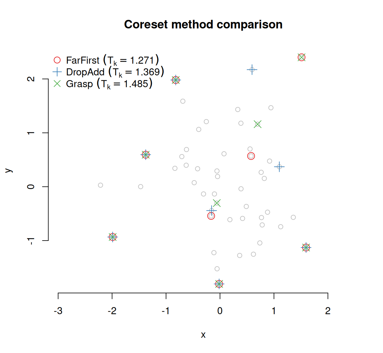

Selections returned by each method on 50 random 2-D points (k = 8). Coloured symbols mark selected points; grey circles are the full candidate set.

Exact solution

For small instances (roughly N ≤ 25–30), ExactMaxMin() solves the problem to proven optimality via a node-packing integer programme (Sayyady & Fathi, 2016), using the highs solver (which we must first install).

install.packages("highs")

set.seed(1L)
pts30 <- matrix(rnorm(60L), ncol = 2L)
d30   <- dist(pts30)

exPick <- ExactMaxMin(6L, d30, maxSeconds = 30L)

attr(exPick, "proven")      # TRUE  ⟹  objective is the global optimum
#> [1] TRUE
attr(exPick, "score")
#> [1] 1.616311

# Compare to the greedy heuristic on the same instance
ff30Pick <- FarFirst(6L, d30)
c(exact    = attr(exPick, "score"),
  farFirst = MinDist(d30, ff30Pick))
#>    exact farFirst 
#> 1.616311 1.616311

$proven = TRUE certifies that no selection can achieve a higher T_k. ExactMaxMin() is NP-hard; it is wise to set a time budget once the number of points exceeds ~30 candidates, or to switch to a heuristic method.

Scoring

MinDist() computes the T_k objective for any index set. It accepts a dist object, a square distance matrix, or a coordinate matrix via the points argument:

MinDist(d50, ffPick)                               # from dist
#> [1] 1.271123
MinDist(as.matrix(d50), ffPick)                    # from square matrix
#> [1] 1.271123
MinDist(points = pts, idx = ffPick)                # from coordinates
#> [1] 1.271123

Max-sum diversity and Max-mean dispersion

The Max-Sum Diversity Problem selects the $k$-subset with the highest total pairwise distance. ExactMaxSum() finds an optimal solution via per-node integer-program linearisation (Kuo et al., 1993).

smPick <- ExactMaxSum(6L, d30, maxSeconds = 30L)

attr(smPick, "proven")      # TRUE  ⟹  objective is the global optimum
#> [1] TRUE
attr(smPick, "score")       # total pairwise distance within the selection
#> [1] 41.00517

Where the number of elements is not specified a priori, Max-Sum diversity generalizes to the Max-Mean Dispersion Problem, which maximizes the sum of pairwise distances divided by the number of selected elements.

MaxMean() implements reinforcement-learning tabu search (Nijimbere et al., 2020): each restart constructs a candidate selection, randomly at first, then guided by a Q-learning memory of which elements proved valuable. The selection is refined with a one-flip tabu search that adds or removes a single element at a time. The search continues until its time budget expires.

The objective is only interesting when negative distances occur: otherwise the optimal selection tends to include all points.

set.seed(1)
affinity <- matrix(runif(30L * 30L, min = -10, max = 10), nrow = 30L)
affinity <- (affinity + t(affinity)) / 2   # symmetric
diag(affinity) <- 0

set.seed(1)
mmPick <- MaxMean(affinity, maxSeconds = 2)
mmPick
#> 10 elements (9 11 14 15 19 20 21 24 26 28) selected by MaxMean RLTS, f = 12.14
attr(mmPick, "size")              # the algorithm chose this subset size
#> [1] 10
attr(mmPick, "score")             # achieved mean-dispersion objective
#> [1] 12.1435

MaxMean() chooses the subset size to retaining only the elements that raise the average separation. MeanDist() scores any index set under the same objective, so a hand-picked selection can be compared directly:

MeanDist(affinity, mmPick)        # matches attr(mmPick, "score")
#> [1] 12.1435
MeanDist(affinity, 1:30)          # the full set scores lower
#> [1] -0.342487

Covering: the k-centre problem

The above methods seek to spread the selection such that its members are mutually far apart. The k-centre problem instead minimizes the covering radius $R$, the largest distance from any point to its nearest chosen centre, such that no point of the pool is left far from a representative (González, 1985; Hochbaum & Shmoys, 1985), typically resulting in selections that reach further into the interior of a sample.

Heuristic approach

FarFirst() is the quickest approximation to the K-centres problem. The CDSh algorithm implemented in KCentres() gives a more sophisticated heuristic (García-Díaz et al., 2017; García-Díaz et al., 2019); its solutions are typically within 1–3.5 % of the optimum, compared to ~10% for FarFirst().

centres <- KCentre(4L, eurodist)
labels(eurodist)[centres]
#> [1] "Cologne"    "Copenhagen" "Madrid"     "Rome"
centres
#> 4 centres (6 7 14 19) by CDSh, covering radius <= 1011

KCentreRadius() scores any centre set by its covering radius (lower is better). CDSh covers at least as tightly as the Gonzalez 2-approximation baseline:

ff <- FarFirst(4L, eurodist, strategy = "peripheral")
c(KCentre  = KCentreRadius(eurodist, centres),
  FarFirst = KCentreRadius(eurodist, ff))
#>  KCentre FarFirst 
#>     1011     1209

Like MinDist(), KCentreRadius() accepts a points coordinate matrix, allowing it to score a selection on a set of points whose distance matrix would be too large to fit in memory.

Exact solver

For small instances, ExactKCentre() finds the optimal solution, using a minimum-set-cover integer program approach akin to ExactMaxMin(), and using again the highs solver.

kc <- ExactKCentre(4L, eurodist)
kc
#> 4 centres (6 7 14 19) by exact cover search, proven optimal, covering radius = 1011
attr(kc, "proven")      # TRUE  ⟹  radius is the global covering optimum
#> [1] TRUE

The covering optimum is sometimes attained by fewer centres (once every point is covered, extra centres cannot lower the radius); indices then has length below the requested number, and the reported radius is still the proven optimum. ExactKCentre() is NP-hard, so — like ExactMaxMin() — it is a ground-truth reference for small instances, not a scalable method.

The dispersion and covering optima differ even on this small example: dispersion selects cities at the rim of the map, while covering pulls inward to keep every city near a centre.

disp <- ExactMaxMin(4L, eurodist)
labels(eurodist)[disp]  # dispersion: pushed to the extremes
#> [1] "Athens"    "Lisbon"    "Milan"     "Stockholm"
labels(eurodist)[kc]    # covering: pulled toward the interior
#> [1] "Cologne"    "Copenhagen" "Madrid"     "Rome"

Maximum-entropy (maxdet) selection

The maximum entropy selection seeks to select $k$ elements that contain as much of the information of the original set as possible. The route to doing so is dropping elements that are redundant to selected elements. If redundancy between two points is equated to the overlap of volumes centred on each point, then maximum entropy can be cast as finding a selection that maximizes the log-determinant of its kernel block, $\log\det K_S$ (Shewry & Wynn, 1987), equivalently the maximum-a-posteriori mode of a determinantal point process (Kulesza & Taskar, 2012).

MaxEntropy() builds a radial-basis kernel from the distance matrix. This is repaired to be positive semi-definite where needed, since an arbitrary distance is not guaranteed to be of negative type.

mePick <- MaxEntropy(4L, eurodist)
labels(eurodist)[mePick]
#> [1] "Athens"    "Geneva"    "Lisbon"    "Stockholm"
attr(mePick, "score")     # the achieved log-determinant
#> [1] 0.02885061
attr(mePick, "exact")      # TRUE if certified by exact enumeration
#> [1] TRUE

The selection is built greedily by pivoted Cholesky, substituting exact enumeration when $\binom{n}{k}$ does not exceed maxCombos. negMass reports the fraction of spectral mass removed by the positive-semidefinite repair; as this fraction increases, so the result must be considered more approximate.

attr(mePick, "negMass")
#> [1] 0.04210186

When to use which method

For dispersion (spread the selection; maximize T_k):

Scenario	Recommended
Speed matters most	`FarFirst()` (ensemble default)
Deterministic, good quality valued	`DropAdd()`
Best quality, `set.seed()` for reproducibility	`Grasp()`
N > 46 000 (distance matrix infeasible)	`DropAdd(points = ...)` or `FarFirst(points = ...)`
Arbitrary metric with no coordinate embedding	`FarFirst(<column function>, N = ...)`
Proven optimum, N ≤ ~ 25–30, highs installed	`ExactMaxMin()`
Score a selection’s T_k	`MinDist()`

For total dispersion (fixed-size subset maximizing the sum of pairwise distances):

Scenario	Recommended
Proven optimum, N ≤ ~ 25–30, highs installed	`ExactMaxSum()`

For average dispersion (select a subset of the size that maximizes mean separation):

Scenario	Recommended
Maximize mean pairwise distance, size unfixed	`MaxMean()`
Distances may be negative	`MaxMean()`
Score a selection’s max-mean objective	`MeanDist()`

For covering (minimise the radius; no point far from a centre):

Scenario	Recommended
Near-optimal covering, fast and deterministic	`KCentre()` (CDSh)
Quick 2-approximation baseline	`FarFirst(strategy = "peripheral")`
Proven optimum, small N	`ExactKCentre()`
Score a centre set’s covering radius (matrix-free at large N)	`KCentreRadius(points = ...)`

For maximum-entropy (maxdet) selection (density-blind volume maximization):

Scenario	Recommended
Maximize spanned volume / avoid near-duplicate selections	`MaxEntropy()`
Proven optimum, `choose(n, k)` small	`MaxEntropy(exact = TRUE)`

Coreset selects a subset from a given set of elements. Several established packages solve neighbouring objectives:

k-medoids / k-median selects elements that minimize the mean distance from each element to its nearest centre. Implementations include:
- cluster::pam(): generates the full O(N²) dissimilarity matrix, and hence caps at n ≤ 65 536;
- banditpam, a matrix-free $O(N \log N)$ implementation restricted to coordinate data;
- cluster::clara() (PAM / FastPAM / FasterPAM);
- ClusterR::Cluster_Medoids().
k-means (stats::kmeans()) selects elements so as to minimize the within-cluster sum of squares around centres that are coordinate means, not data points; as such, it applies only to Euclidean coordinates. k-means++ (TreeDist::KMeansPP()) initializes its selection using D²-weighted seeding, a randomized relative of FarFirst()’s farthest-first traversal.
maximin solves the related design problem of adding new points at positions that maximize the minimum inter-point distance.

References

García-Díaz, J., Menchaca-Méndez, R., Menchaca-Méndez, R., Pomares Hernández, S., Pérez-Sansalvador, J. C., & Lakouari, N. (2019). Approximation algorithms for the vertex $k$-center problem: Survey and experimental evaluation. IEEE Access, 7, 109228–109245. https://doi.org/10.1109/ACCESS.2019.2933875

García-Díaz, J., Sánchez-Hernández, J., Menchaca-Méndez, R., & Menchaca-Méndez, R. (2017). When a worse approximation factor gives better performance: A 3-approximation algorithm for the vertex $k$-center problem. Journal of Heuristics, 23(5), 349–366. https://doi.org/10.1007/s10732-017-9345-x

González, T. F. (1985). Clustering to minimize the maximum intercluster distance. Theoretical Computer Science, 38, 293–306. https://doi.org/10.1016/0304-3975(85)90224-5

Hochbaum, D. S., & Shmoys, D. B. (1985). A best possible heuristic for the $k$-center problem. Mathematics of Operations Research, 10(2), 180–184. https://doi.org/10.1287/moor.10.2.180

Kulesza, A., & Taskar, B. (2012). Determinantal point processes for machine learning. Foundations and Trends in Machine Learning, 5(2–3), 123–286. https://doi.org/10.1561/2200000044

Kuo, C.-C., Glover, F., & Dhir, K. S. (1993). Analyzing and modeling the maximum diversity problem by zero-one programming. Decision Sciences, 24(6), 1171–1185. https://doi.org/10.1111/j.1540-5915.1993.tb00509.x

Nijimbere, D., Zhao, S., Gu, X., Esangbedo, M. O., & Dominique, N. (2020). Tabu search guided by reinforcement learning for the max-mean dispersion problem. Journal of Industrial & Management Optimization, 17, 3223–3254. https://doi.org/10.3934/jimo.2020115

Porumbel, D., Hao, J.-K., & Glover, F. (2011). A simple and effective algorithm for the MaxMin diversity problem. Annals of Operations Research, 186, 275–293. https://doi.org/10.1007/s10479-011-0898-z

Resende, M. G. C., Martí, R., Gallego, M., & Duarte, A. (2010). GRASP and path relinking for the max-min diversity problem. Computers & Operations Research, 37(3), 498–508. https://doi.org/10.1016/j.cor.2008.05.011

Sayyady, F., & Fathi, Y. (2016). An integer programming approach for solving the p-dispersion problem. European Journal of Operational Research, 253(1), 216–225. https://doi.org/10.1016/j.ejor.2016.02.026

Shewry, M. C., & Wynn, H. P. (1987). Maximum entropy sampling. Journal of Applied Statistics, 14(2), 165–170. https://doi.org/10.1080/02664768700000020