Extending the Robinson-Foulds metric

The Robinson–Foulds distance

An intuitive way to calculate the similarity between two trees is to calculate the resolution of their strict consensus, which corresponds to the number of splits that occur in both trees (Schuh & Polhemus, 1980). The corresponding distance measure, the Robinson–Foulds distance (Robinson & Foulds, 1981), counts the number of splits that are unique to one of the two trees.

It is important to remember that counting splits is not the same as counting clades, edges or nodes. If a tree is drawn as rooted (even without a root edge), then the number of splits is one less than the number of edges or clades, and two less than the number of nodes. For example, the trees below have one split, two edges and three nodes in common.

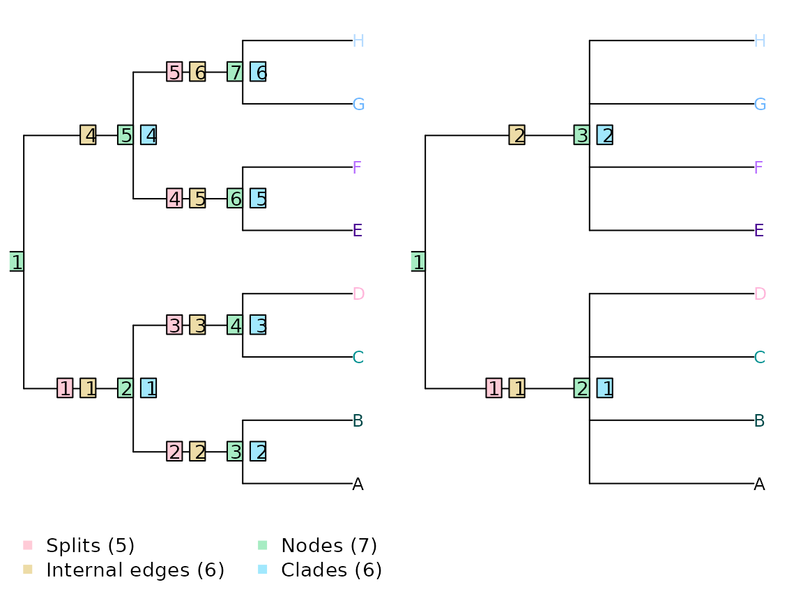
The simplicity of counting splits is appealing, but limited by the underlying assumption that all splits are equivalent.

As an example, a split that separates eight leaves into two sets of four (as in the right-hand tree above) has a $\frac{1}{35}$ chance of being compatible with the reference tree. In contrast, a split that separates two leaves from the other six has a $\frac{1}{7}$ chance of matching the reference tree: the similarity observed is five times more likely to have arisen by chance. In other words, failure to match an even split is less noteworthy than failure to match an uneven one.

As a consequence, trees whose splits are less even will, on average, exhibit higher Robinson–Foulds distances with comparison trees. Compare a balanced and an unbalanced eight-taxon tree:

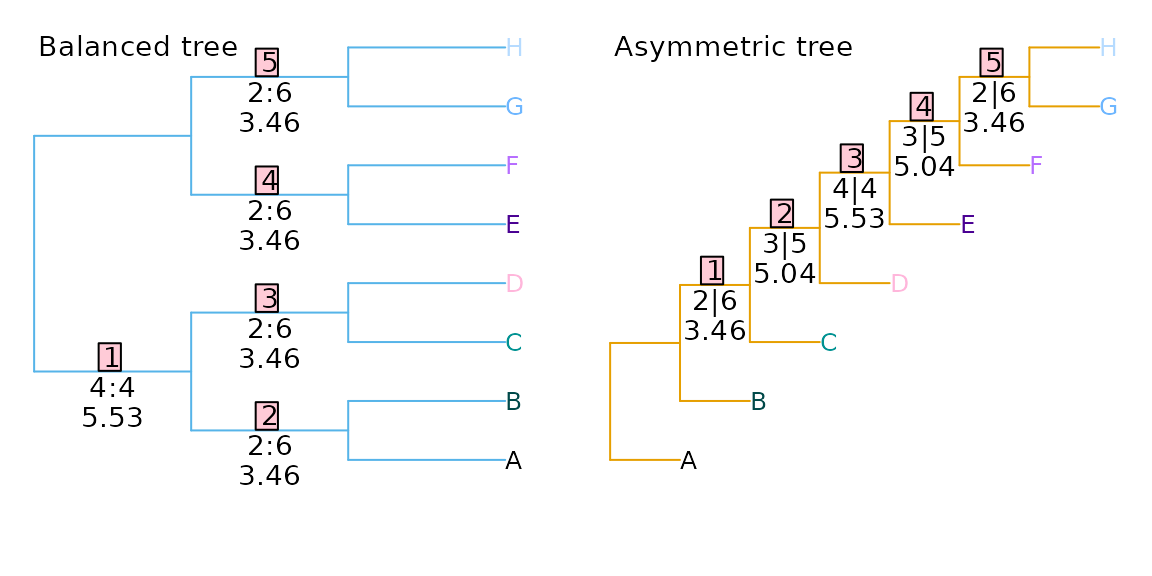
Each tree divides the eight taxa into five splits. The phylogenetic information content of a split is a function of the probability that the split will match a uniformly chosen random tree, i.e. the proportion of eight-leaf binary trees that contain the split in question. (Information content, in bits, is defined as $-\log_2(\textrm{probability})$ .) This, in turn, is a function of the evenness of the split:

	Matching trees	P(Match in random tree)	Phylogenetic information content
Split size: 2:6	945 / 10 395	0.0909	3.46 bits
Split size: 3:5	315 / 10 395	0.0303	5.04 bits
Split size: 4:4	225 / 10 395	0.0216	5.53 bits

In the first tree, split 1 is even, dividing four taxa from four others (4|4); splits 2–5 are maximally uneven (2|6). If each split is treated as independent, then the total information content of the five splits is 19.37 bits, whereas that of the five splits in the second tree, of sizes 2|6, 3|5, 4|4, 3|5 and 2|6, is 22.54 bits. Put another way, a random tree will on average share more splits with the balanced tree (whose splits are predominantly uneven and thus likely to be matched) than the asymmetric tree (which contains more even splits that are less likely to occur in a random tree).

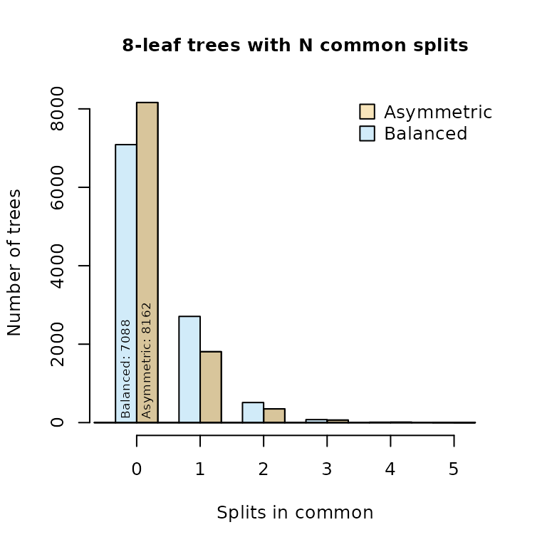
Indeed, of the 10 395 eight-leaf trees, many more bear at least one split in common with a balanced tree than with an asymmetric tree:

Information-corrected Robinson–Foulds distance

This differing information content can be accommodated by weighting each split according to the amount of phylogenetic information it contains (Smith, 2020). The two tree pairs below both have a Robinson–Foulds distance of two, but the first pair differ with regard to an uneven split (ABCDEF|GH), so obtain a total difference of 22.54 − (3.46 + 5.04 + 5.53 + 5.04) = 3.46 bits:

tree1 <- ape::read.tree(text='(1, (2, (3, (4, (5, (6, (7, 8)))))));')
tree2 <- ape::read.tree(text='(1, (2, (3, (4, (5, (7, (6, 8)))))));')
tree3 <- ape::read.tree(text='(1, (2, (3, (5, (4, (6, (7, 8)))))));')

VisualizeMatching(InfoRobinsonFoulds, tree1, tree2, 
                  Plot = TreeDistPlot, prune = 12)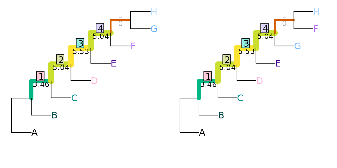

whereas the second pair differ in the resolution of a more even, and thus more information-rich, split (ABCD|EFGH), and so receive a distance score of 5.53 bits:

VisualizeMatching(InfoRobinsonFoulds, tree1, tree3, 
                  Plot = TreeDistPlot, prune = 8)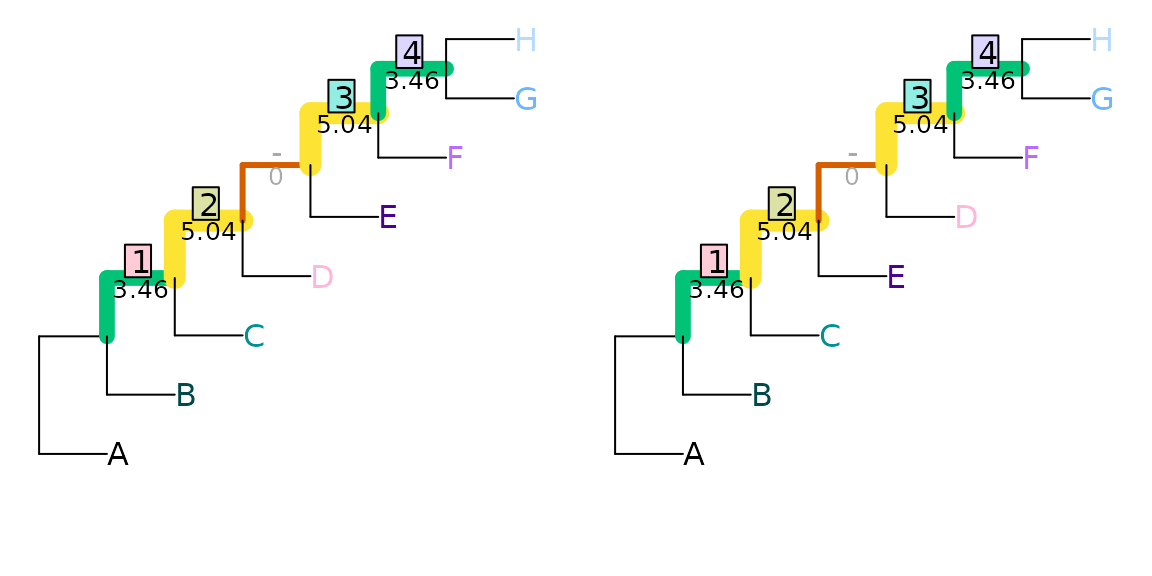

Generalized Robinson–Foulds distances

Even when accounting for the information content of splits in this way, the Robinson–Foulds distance is readily saturated: the maximum value can be obtained by moving a single leaf.

tree1 <- ape::read.tree(text='(1, (2, (3, (4, (5, (6, (7, 8)))))));')
tree2 <- ape::read.tree(text='(8, (1, (2, (3, (4, (5, (6, 7)))))));')

VisualizeMatching(RobinsonFouldsMatching, tree1, tree2, Plot = TreeDistPlot)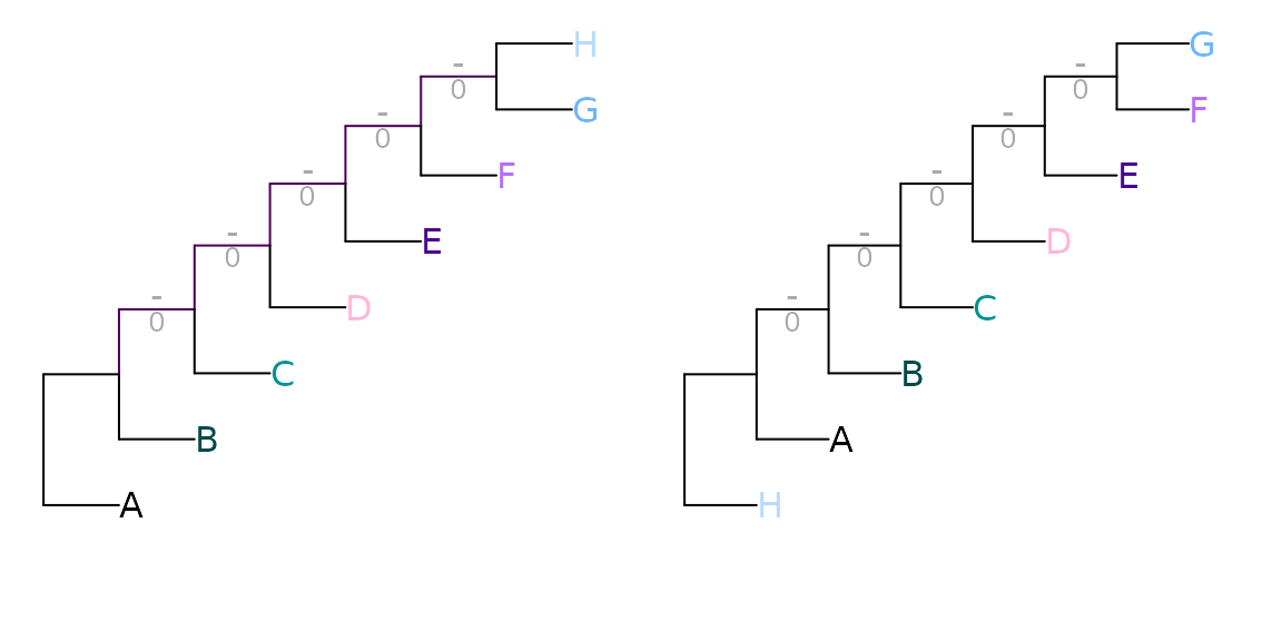

Generalized Robinson–Foulds distances (Böcker, Canzar, & Klau, 2013; Nye, Liò, & Gilks, 2006) seek to address this issue. This category of metrics aim to acknowledge semblances between similar-but-not-quite-identical pairs of splits, which would contribute zero to tree similarity under the standard Robinson–Foulds measure.

Generalized RF distances work by finding a matching that pairs splits from one tree with splits in the other. Each pairing is scored according to the similarity of the paired splits; the sum of these scores is the score of the matching. The tree distance is given by the score of the optimal matching.

Constructing a matching

Let’s consider two trees that differ in the position of one wildcard leaf, and in the resolution of a clade:

tree1 <- ape::read.tree(text='((A, B), ((C, (D, E)), (F, (G, (H, I)))));')
tree2 <- ape::read.tree(text='((A, B), ((C, D, (E, I)), (F, (G, H))));')

Plot(tree1, tree2, highlight = 'I', prune = list(8, integer(0)))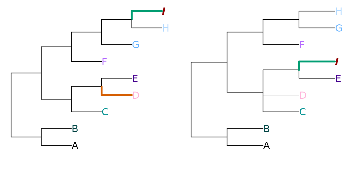

These trees obtain a Robinson–Foulds distance of nine: a large distances, as the maximum possible for trees of this resolution is eleven. AB|CDEFGHI is the only split in common between the two trees:

TwoTreePlot()
VisualizeMatching(RobinsonFouldsMatching, tree1, tree2)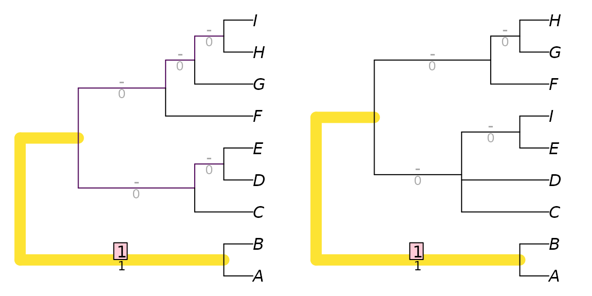

This distance score is higher than might be expected, given how much the trees have in common; removing the single leaf ‘I’ results in two trees that differ only in the resolution of a single node:

TwoTreePlot()
VisualizeMatching(RobinsonFouldsMatching,
                  drop.tip(tree1, 'I'),
                  drop.tip(tree2, 'I'))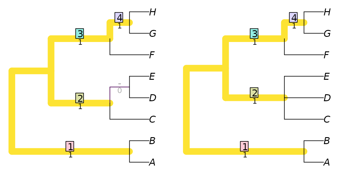

This hidden similarity can be better reflected if similar, but non-identical, splits are assigned non-zero similarity scores.

There are various ways to score the similarity between two splits. One is to build on the idea introduced above, where identical splits are scored according to their phylogenetic information content. Non-matching splits can be scored according to the amount of phylogenetic information that they hold in common, which is a function of the proportion of trees that are consistent with both splits. (A full explanation is provided in the discussion of Generalized Robinson–Foulds distances.)

TwoTreePlot()
VisualizeMatching(SharedPhylogeneticInfo, tree1, tree2)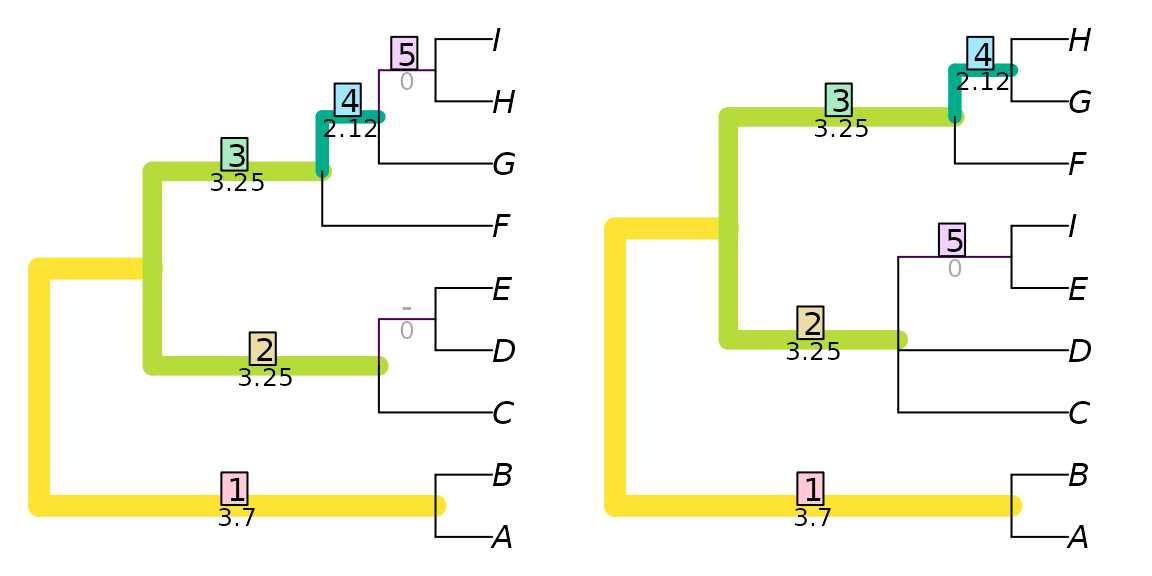

Here, the split AB|CDEFGHI occurs in both trees, and, as it happens, makes the largest contribution to the tree similarity score (3.70) for this particular pair of trees. This is the same contribution it would have made to the information-corrected Robinson–Foulds similarity.

The split ABCDEF|GHI in the left-hand tree is paired with the split ABCDEFI|GH in the right-hand tree. Had ABCDEF|GHI been available in the right-hand tree, then this perfect match would have been assigned a similarity of SplitInformation(3, 6) = 5.57 bits. The partial match is instead allocated a lower score of 2.12 bits. Pairings of incompatible splits, i.e. those that cannot co-exist on a tree, such as ABCDEFG|HI - ABCDFGH|EI, have no phylogenetic information in common. (clustering information is an alternative way to think about split similarity that recognizes similarity even between incompatible splits.)

The matching depicted above is one of many. It happens to be optimal: an optimal matching can be found by considering the similarity score of each possible pairing, and solving a linear assignment problem to find the optimal set of pairings.

We can view the splits in each tree, named according to the number of their associated node:

summary(TreeTools::as.Splits(tree1, LETTERS[1:9]))

## 6 bipartition splits dividing 9 tips, A .. I
##      123456789
##  11  **.......
##  13  ..***....
##  14  ...**....
##  15  .....****
##  16  ......***
##  17  .......**
## 
##  Tip 1: A     Tip 2: B    Tip 3: C    Tip 4: D    Tip 5: E   
##  Tip 6: F     Tip 7: G    Tip 8: H    Tip 9: I

summary(TreeTools::as.Splits(tree2, LETTERS[1:9]))

## 5 bipartition splits dividing 9 tips, A .. I
##      123456789
##  11  **.......
##  13  ..***...*
##  14  ....*...*
##  15  .....***.
##  16  ......**.
## 
##  Tip 1: A     Tip 2: B    Tip 3: C    Tip 4: D    Tip 5: E   
##  Tip 6: F     Tip 7: G    Tip 8: H    Tip 9: I

We can then see the similarity scores for each pair of splits, along with the optimal matching:

attributes(SharedPhylogeneticInfo(tree1, tree2, reportMatching = TRUE))

## $matching
## [1]  1  2 NA  4  5  3
## 
## $matchedSplits
## [1] "A B | C D E F G H I => A B | C D E F G H I"
## [2] "C D E | A B F G H I => C D E I | A B F G H"
## [3] "F G H I | A B C D E => F G H | A B C D E I"
## [4] "G H I | A B C D E F => G H | A B C D E F I"
## [5] "H I | A B C D E F G .. E I | A B C D F G H"
## 
## $matchedScores
## [1] 3.700440 3.252981       NA 3.252981 2.115477 0.000000
## 
## $pairScores
##           [,1]      [,2]      [,3]      [,4]      [,5]
## [1,] 3.7004397 0.8930848 0.2410081 0.5305147 0.2410081
## [2,] 0.5305147 3.2529807 0.0000000 1.1825914 0.5305147
## [3,] 0.2410081 1.3785116 0.0000000 0.5305147 0.2410081
## [4,] 0.8930848 0.0000000 0.0000000 3.2529807 1.3785116
## [5,] 0.5305147 0.0000000 0.0000000 0.0000000 2.1154772
## [6,] 0.2410081 0.0000000 0.0000000 0.0000000 0.0000000

.. denotes that the fifth matching contributes zero to similarity score; an alternative optimal matching would leave these splits unpaired.

What next?

Alternatives measures of split similarity, such as mutual clustering information, give rise to other Generalized Robinson–Foulds distances, and can be used to generate meaningful tree spaces.

References

Böcker, S., Canzar, S., & Klau, G. W. (2013). The generalized Robinson-Foulds metric. In A. Darling & J. Stoye (Eds.), Algorithms in Bioinformatics. WABI 2013. Lecture Notes in Computer Science, vol 8126 (pp. 156–169). Berlin, Heidelberg: Springer. doi:10.1007/978-3-642-40453-5_13

Nye, T. M. W., Liò, P., & Gilks, W. R. (2006). A novel algorithm and web-based tool for comparing two alternative phylogenetic trees. Bioinformatics, 22(1), 117–119. doi:10.1093/bioinformatics/bti720

Robinson, D. F., & Foulds, L. R. (1981). Comparison of phylogenetic trees. Mathematical Biosciences, 53(1-2), 131–147. doi:10.1016/0025-5564(81)90043-2

Schuh, R. T., & Polhemus, J. T. (1980). Analysis of taxonomic congruence among morphological, ecological and biogeographic data sets for the Leptopodomorpha (Hemiptera). Systematic Biology, 29(1), 1–26. doi:10.1093/sysbio/29.1.1