Analysing landscapes of phylogenetic trees

Landscapes of trees are mappings of tree space that are contoured according to some optimality criterion – often, but not necessarily, a tree’s score under a phylogenetic reconstruction technique (Bastert et al., 2002). Detecting “islands” or “terraces” of trees can illuminate the nature of the space of optimal trees and thus inform tree search strategy (Maddison, 1991; Sanderson et al., 2011).

For simplicity (and to avoid scoring trees against a dataset), this example uses a tree’s balance (measured using the total cophenetic index) as its score (Mir et al., 2013). We assume that mappings have already been shown to be adequate (Smith, 2022).

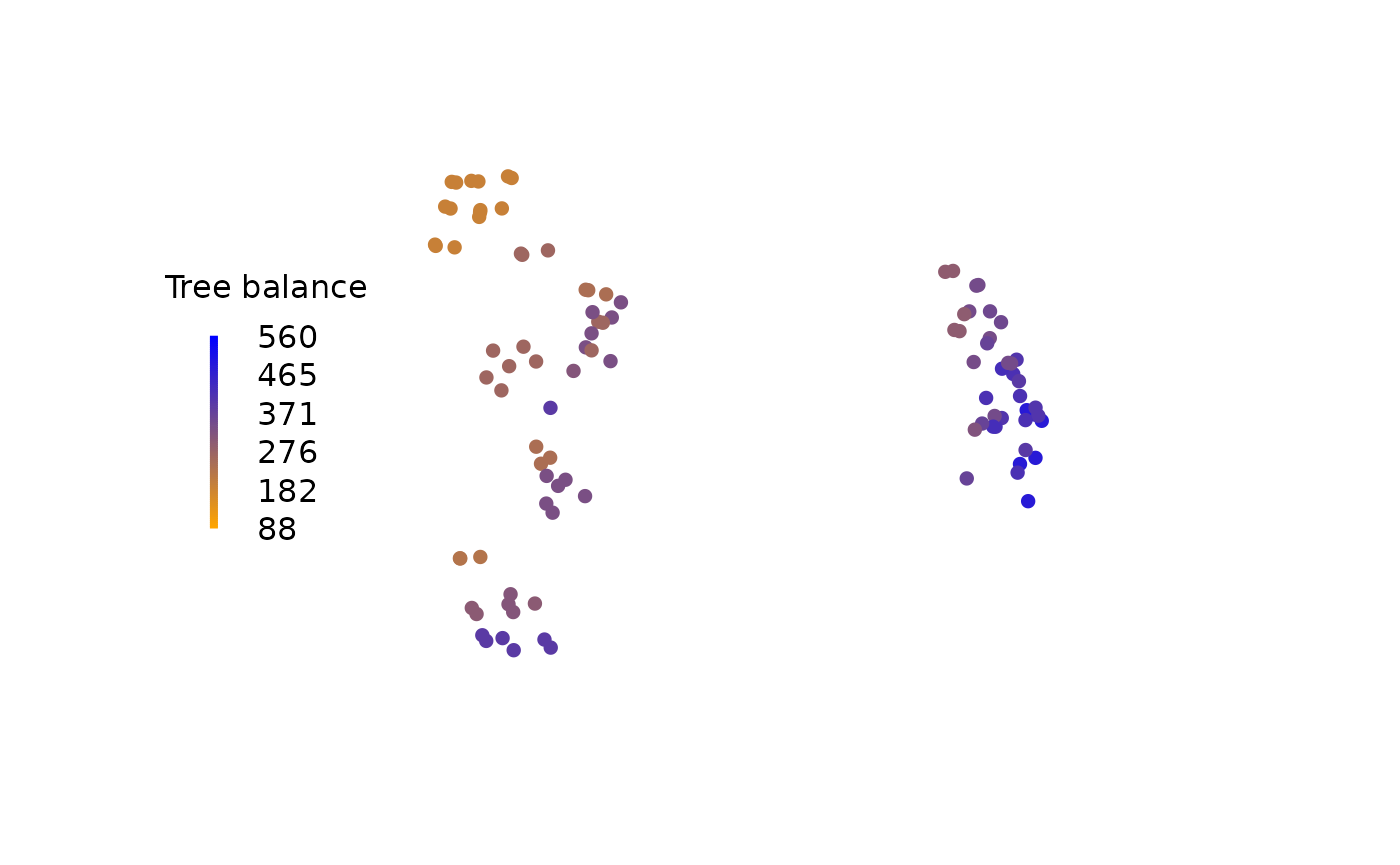
A landscape is most simply visualized by colouring each tree according to its score:

# Load required libraries
library("TreeTools", quietly = TRUE)
library("TreeDist")

# Generate a set of trees
trees <- as.phylo(as.TreeNumber(BalancedTree(16)) + 0:100 - 15, 16)

# Create a 2D mapping
distances <- ClusteringInfoDist(trees)
mapping <- cmdscale(distances, 2)

# Score trees according to their balance
scores <- TotalCopheneticIndex(trees)

# Normalize scores
scoreMax <- TCIContext(trees[[1]])[["maximum"]]
scoreMin <- TCIContext(trees[[1]])[["minimum"]]
scores <- scores - scoreMin
scores <- scores / (scoreMax - scoreMin)

# Generate colour palette
col <- colorRamp(c("orange", "blue"))(scores)
rgbCol <- rgb(col, maxColorValue = 255)

# Plot trees, coloured by their score
plot(
  mapping,
  asp = 1, # Preserve aspect ratio - do not distort distances
  ann = FALSE, axes = FALSE, # Don't label axes: dimensions are meaningless
  col = rgbCol, # Colour trees by score
  pch = 16 # Plotting character: Filled circle
)

# Add a legend
PlotTools::SpectrumLegend(
  "left",
  title = "Tree balance",
  palette = rgb(colorRamp(c("orange", "blue"))(0:100 / 100) / 255),
  legend = floor(seq(scoreMax, scoreMin, length.out = 6)),
  bty = "n"
)

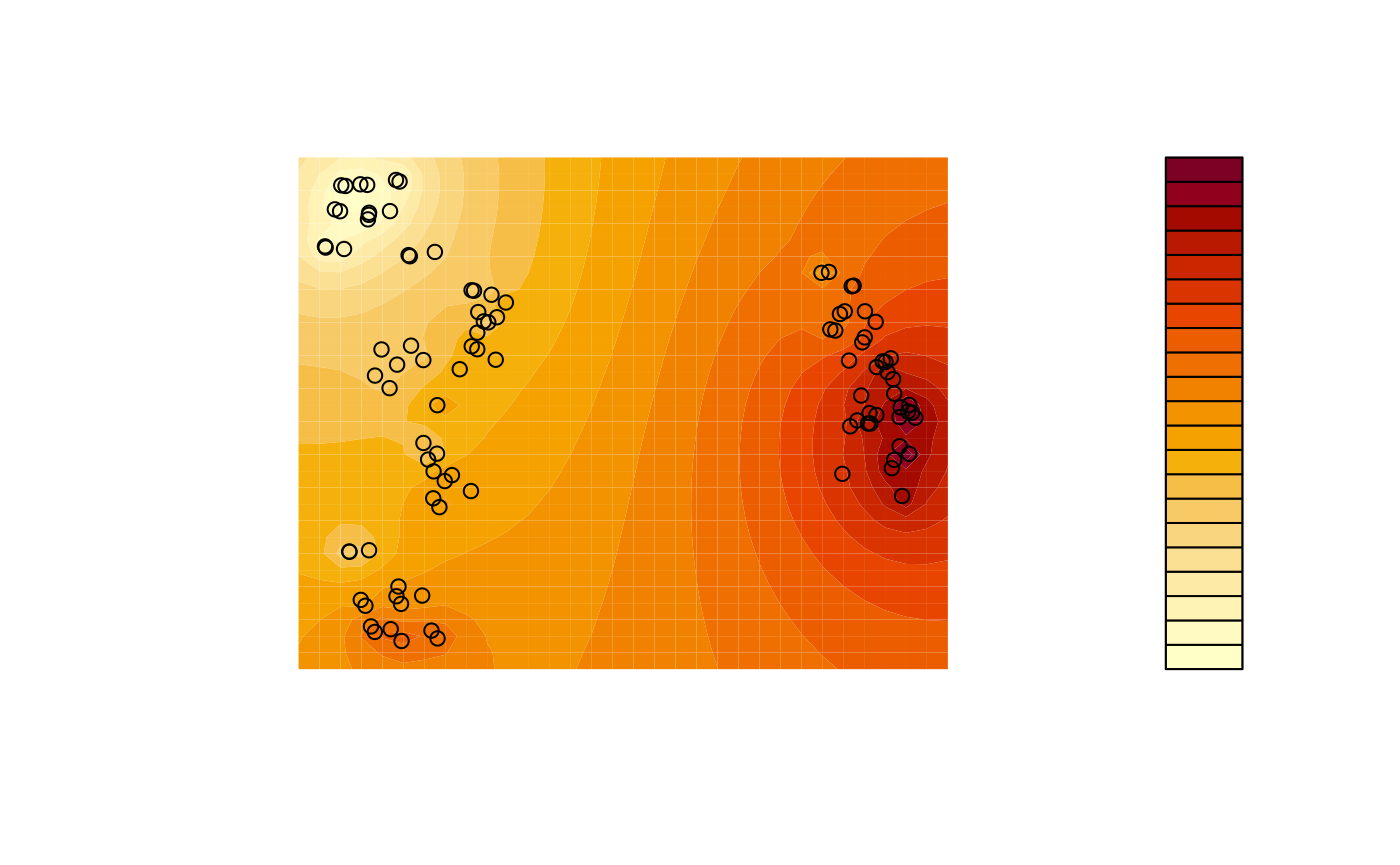
A more sophisticated output can be produced using contours, interpolating between adjacent trees. This example uses a simple inverse distance weighting function for interpolation; more sophisticated techniques such as kriging or (in continuous tree spaces) the use of geodesics (Khodaei et al., 2022) can produce even better results.

# Use an inverse distance weighting to interpolate between measured points
Predict <- function (x, y) {
  Distance <- function (a, b) {
    apply(a, 2, function (pt) sqrt(colSums((pt - b) ^ 2)))
  }
  predXY <- rbind(x, y)
  dists <- Distance(t(mapping), predXY)
  invDist <- 1 / dists
  weightings <- invDist / rowSums(invDist)

  # Return:
  colSums(scores * t(weightings))
}

# Generate grid for contour plot
resolution <- 32
xLim <- range(mapping[, 1]) * 1.1
yLim <- range(mapping[, 2]) * 1.11
x <- seq(xLim[1], xLim[2], length.out = resolution)
y <- seq(yLim[1], yLim[2], length.out = resolution)
z <- outer(x, y, Predict) # Predicted values for each grid square

# Plot
filled.contour(
  x, y, z,
  asp = 1, # Preserve aspect ratio - do not distort distances
  ann = FALSE, axes = FALSE, # Don't label axes: dimensions are meaningless
  plot.axes = {points(mapping, xpd = NA)} # Use filled.contour coordinates
)

A variety of R add-on packages facilitate three-dimensional plots.

if (requireNamespace("plotly", quietly = TRUE)) {
  library("plotly", quietly = TRUE)
  fig <- plot_ly(x = x, y = y, z = z)
  fig <- fig %>% add_surface()
  fig
} else {
  print("Run `install.packages('plotly')` to view this output")
}

(Use the mouse to reorient)

References

Bastert, O., Rockmore, D., Stadler, P. F., & Tinhofer, G. (2002). Landscapes on spaces of trees. Applied Mathematics and Computation, 131(2-3), 439–459. https://doi.org/10.1016/S0096-3003(01)00164-3

Khodaei, M., Owen, M., & Beerli, P. (2022). Geodesics to characterize the phylogenetic landscape. bioR $\chi$ iv. https://doi.org/10.1101/2022.05.11.491507

Maddison, D. R. (1991). The discovery and importance of multiple islands of most-parsimonious trees. Systematic Biology, 40(3), 315–328. https://doi.org/10.1093/sysbio/40.3.315

Mir, A., Rosselló, F., & Rotger, L. A. (2013). A new balance index for phylogenetic trees. Mathematical Biosciences, 241(1), 125–136. https://doi.org/10.1016/j.mbs.2012.10.005

Sanderson, M. J., McMahon, M. M., & Steel, M. (2011). Terraces in Phylogenetic Tree Space. Science, 333(6041), 448–450. https://doi.org/10.1126/science.1206357

Smith, M. R. (2022). Robust analysis of phylogenetic tree space. Systematic Biology, 71(5), 1255–1270. https://doi.org/10.1093/sysbio/syab100

Martin R. Smith

References