About the quartet distance
Martin R. Smith
2026-06-15
Source:vignettes/Quartet-Distance.Rmd
Quartet-Distance.RmdPartition distances
The Robinson-Foulds (RF or ‘partition’) metric (Robinson & Foulds, 1981; Steel & Penny, 1993) measures the symmetric difference between two trees by adding the number of splits (i.e. groupings) that are present in tree A (but not tree B) to the number of splits present in tree B (but not tree A).
It is most useful when the trees to be compared are very similar; it has a low range of integer values, and a low maximum value, limiting its ability to distinguish between trees (Steel & Penny, 1993); and it treats all splits as equivalent, even though some are more informative than others. Various other artefacts and biases limit its performance against a suite of real-world benchmarks (Smith, 2020, 2022). These shortcomings can largely be mitigated through generalizations of the Robinson-Foulds distance (see R package ‘TreeDist’), but the complementary perspective on tree similarity offered by a quartet-centred approach can be illuminating.
Quartet distances
Instead of partitions, symmetric differences can be measured by counting the number of four-taxon statements (quartets) that differ between two trees (Day, 1986; Estabrook et al., 1985).
For any four tips A, B, C and D, a split on a bifurcating tree will separate tip A and either B, C or D from the other two tips. That is to say, removing all other tips from the tree will leave one of these three trees:
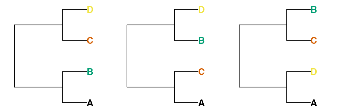
Thus two of the random trees below share the quartet
(A, B), (C, D), whereas the third does not; these four tips
are divided into (A, D), (B, C).
There are groups of four taxa in a tree with tips; for each of these groups, one of the three trees above will be consistent with a given tree. As such, two identical trees will have a quartet distance of 0, and a random pair of trees will have an expected quartets in common. Because quartets are not independent of one another, no pair of trees with six or more tips can have all quartets in common (Steel & Penny, 1993).
Properties of the quartet distance are explored fully in Steel & Penny (1993). As quartet distances of 1 can only be accomplished for small trees (five or fewer leaves; see below), it is perhaps more appropriate to consider whether or not trees are more dissimilar than a pair of random trees, whose distance will be, on average, . (Data from real trees, and comparisons with expected values of other metrics, are available (here)[https://ms609.github.io/TreeDistData/articles/09-expected-similarity.html].)
Normalization
Whereas counting quartets is simple, accounting for resolution is
not. Two trees will have few quartet statements in common if they are
well resolved and differ in many details; or if they are poorly resolved
but in perfect agreement. As such, it is important to normalize quartet
distances in a meaningful fashion. A number of normalizations have been
proposed (Day, 1986; Estabrook et al.,
1985); arguably the most appropriate is the Symmetric Quartet
Divergence (Smith, 2019), which represents
the total number of quartets unique to each tree normalized against the
total number of quartets that could have been resolved. The
SimilarityMetrics() documentation page gives further
details.
Asymmetric differences
Metric distances are necessarily symmetric – that is, the distance from tree A to tree B equals the distance from B to A. This behaviour is not necessarily desirable when one tree represents a known ‘reference’ – such as a tree validated by independent data, or a tree used to simulate data in order to test phylogenetic reconstruction techniques.
In such cases, a tree might be evaluated according to the likelihood
that a randomly chosen quartet is resolved correctly by the tree, where
an uncertain resolution in either the reference or comparison tree is
taken as having a 1/3 chance of being correct (Asher & Smith
forthcoming). More details are given at the
SimilarityMetrics() documentation page.
Quartet similarity in a pair of random trees
On average, of the quartets resolved in a pair of random trees will match. This is because there are three quartets involving any set of four tips, each of which is equally likely to occur on a truly random tree.
The below code calculates the mean proportion of matching quartets between 10 random trees (90 pairs) with 4 to 20 leaves, and the corresponding standard deviation.
round(vapply(4:20, function (nTip) {
 trees <- lapply(rep(nTip, 10), TreeTools::RandomTree)
 s <- ManyToManyQuartetAgreement(trees)[, , 's']
 results <- s[lower.tri(s)] / choose(nTip, 4)
 c(mean(results), sd(results))
}, c(mean = 0, sd = 0)), 3)
## [,1] [,2] [,3] [,4] [,5] [,6] [,7] [,8] [,9] [,10] [,11] [,12]
## mean 0.311 0.378 0.311 0.367 0.347 0.317 0.334 0.359 0.346 0.329 0.343 0.339
## sd 0.468 0.257 0.194 0.157 0.112 0.087 0.092 0.106 0.080 0.061 0.066 0.049
## [,13] [,14] [,15] [,16] [,17]
## mean 0.335 0.34 0.344 0.340 0.339
## sd 0.044 0.06 0.048 0.045 0.029Independence
One possible criticism of the quartet distance is that not all
individual quartet statements are independent. For example, the quartet
statements AB | CD and AB | CE together imply
AB | DE. A simple count of identical quartets therefore
includes some redundant information. This prevents a straightforward
information theoretic interpretation of the quartet distance.
Minimum quartet similarity
As a related phenomenon, when there are six or more tips in a bifurcating tree, some quartets are necessarily shared between trees.
Consider the tree:
tree_a <- ape::read.tree(text = "((1, 2), (3, (4, 5)));")
The only trees with no quartets in common with Tree A are symmetric with
tree_b <- ape::read.tree(text = "((1, 5), (3, (2, 4)));")
Now create Tree C by adding a 6th tip as a sister to tip
3 on Tree A.
tree_c <- ape::read.tree(text="((1, 2), ((3, 6), (4, 5)));")
There’s nowhere to add tip 6 to Tree B without creating
a quartet that exists in Tree C.
As such, the minimum possible quartet similarity is non-zero, and becomes increasingly difficult to compute as the number of leaves rises. This fact increases the value of comparing low quartet similarity scores to the expected similarity of a pair of random trees (i.e. ), rather than to zero.