Getting started: Exploring tree space
Martin R. Smith
2026-04-23
Source:vignettes/tree-space.Rmd
tree-space.RmdMapping the distribution of trees in “tree space” can reveal patterns in the set of optimal trees, and allow additional details to be obtained from results that may appear to lack resolution (Smith, 2022a).
The ‘TreeSearch’ GUI allows rapid visualisation of tree spaces and the construction of cluster consensus trees, to depict the underlying structure inherent in a set of optimal trees.
More detailed tree space analysis can also be conducted using the ‘TreeDist’ package.
Loading trees into the GUI
This example uses the Sun et al. (2018) dataset included with the TreeSearch package, which contains trees generated under four optimality criteria. The approach will work on search results generated by tree search within the GUI, or any set of trees loaded using the “Load trees” function.
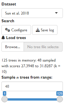
For rapid processing, large tree sets are down-sampled when loaded: here, 48 of the 125 trees are used for analysis. This is useful for obtaining an initial overview of results; including more trees gives a more complete picture but results will take quadratically longer to generate.
If loading the output of a Bayesian analysis, you may wish to modify the range of trees sampled to exclude trees generated during the burn-in phase.

Equivalent R code can be downloaded using the “Save plot: R script” button, and is provided here for reference:
# Load required libraries
library("TreeTools", quietly = TRUE)
library("TreeDist")
library("TreeSearch")


# Load Sun et al. 2018 trees from TreeSearch package
treeFile <- system.file("datasets/Sun2018.nex", package = "TreeSearch")

# Load trees from your own file with
# treeFile <- "Path/to/my.file"
#
# To check and set working directory, use:
# getwd() # Should match location of data / tree files
# setwd(".") # Replace . with desired/directory to change

# Read all trees from file
trees <- read.nexus(treeFile)

# Down-sample to a maximum of 48 trees
trees <- trees[unique(as.integer(seq.int(1, length(trees), length.out = 48)))]
Exploring the consensus
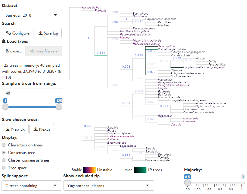
The GUI will initially display the strict consensus of the input trees, after gaining as much information as possible by removing any “rogue” taxa whose position is highly variable (Smith, 2022b).
If trees were generated by a probabilistic sampling process (e.g. Markov Chain) then a majority rule consensus (figure: Majority = 0.5) may reveal additional resolution, but note that the frequency of splits in trees found by parsimony search does not correspond to split support – only the strict consensus tree has any direct interpretation in this setting.

Equivalent R code can be downloaded using the “Save plot: R script” button within the GUI, and is provided here for reference:
# Select an appropriate majority value
# When analysing parsimony results, this value should be 1.
majority <- 0.5

# Identify rogue taxa
exclude <- Rogue::QuickRogue(trees, p = majority)$taxon[-1]
exclude
## [1] "Paterimitra" "Yuganotheca_elegans"
# Select a rogue whose positions should be depicted
plottedRogue <- exclude[1]

# Remove other excluded taxa from tree
consTrees <- lapply(trees, DropTip, setdiff(exclude, plottedRogue))

# Colour tip labels according to their original 'instability' (Smith 2022a)
tipCols <- Rogue::ColByStability(trees)

# Our plotted rogue will not appear on the tree
tipCols <- tipCols[setdiff(consTrees[[1]]$tip.label, plottedRogue)]


# Set up plotting area
par(
 mar = c(0, 0, 0, 0), # Zero margins
 cex = 0.8            # Smaller font size
)

# Plot the reduced consensus tree, showing position of our plotted rogue
plotted <- RoguePlot(
 trees = consTrees,
 tip = plottedRogue,
 p = majority,
 edgeLength = 1,
 tip.color = tipCols
)

# Calculate split concordance
concordance <- SplitFrequency(plotted$cons, trees) / length(trees)

# Annotate splits by concordance
LabelSplits(
 tree = plotted$cons,
 labels = signif(concordance, 3),
 col = SupportColor(concordance),
 frame = "none",
 pos = 3
)
The structure of tree space
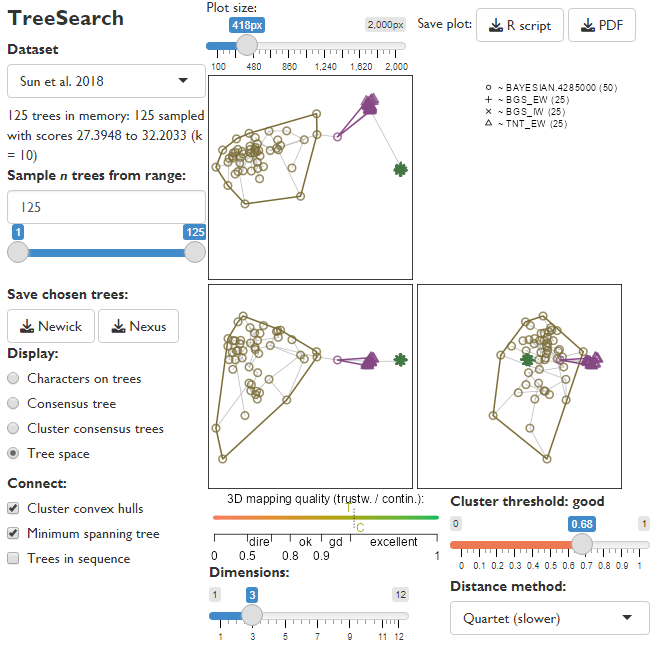
The “Tree space” display option plots trees as points, and attempts to map the distribution of points such that the distance between mapped points corresponds to the tree distance between each pair of trees.
The default method (Clustering Information distance) has many advantages over the widely-used Robinson–Foulds distance (Smith, 2020, 2022a); the quartet distance, whilst slower to calculate, can also produce good low-dimensional mappings of tree space.
The number of dimensions of space can be reduced to make mappings easier to interpret, but do check that the mapping quality gauge remains at least “good”, or perceived structure may be an artefact of distortion.

In this dataset, trees are assigned to three distinct clusters, and display “good” structure: clusters are marked only when their silhouette coefficient is greater than the threshold, whose interpretation is marked above the slider (here, 0.68 is “good”). As it happens, the clusters largely correspond to the tree reconstruction method used: Fitch (1971) parsimony (TNT_EW) trees form one distinct cluster; trees under “BGS” inapplicable-corrected parsimony (Brazeau et al., 2019) another; and Bayesian trees a final, more diffuse cluster.
Tree space analysis in R
More sophisticated tree space analysis can be conducted using the ‘TreeDist’ package.
Sample R code can be downloaded using the “Save plot: R script” button within the GUI, and is provided here for reference:
Generate distances
Different tree distances reflect different aspects of tree similarity, which may or may not be relevant to phylogenetic questions (Smith, 2020, 2022a).
# Compute distances between pairs of trees
dists <- TreeDist::ClusteringInfoDistance(trees)
# The quartet distance is a slower alternative:
library("Quartet")
dists <- as.dist(Quartet::QuartetDivergence(
   Quartet::ManyToManyQuartetAgreement(trees), similarity = FALSE)
)
Identify clustering structure
Here we compute clusters of trees using a selection of clustering methods (Bien & Tibshirani, 2011; Hartigan & Wong, 1979; Maechler et al., 2019), allowing the optimal clustering to be highlighted on the plot.
# Try K-means clustering (Hartigan & Wong 1979):
kClusters <- lapply(
  2:15, # Minimum 2 clusters; maximum 15
  function (k) kmeans(dists, k)
)
kSils <- vapply(kClusters, function (kCluster) {
 mean(cluster::silhouette(kCluster$cluster, dists)[, 3])
}, double(1))
bestK <- which.max(kSils)
kSil <- kSils[bestK] # Best silhouette coefficient
kCluster <- kClusters[[bestK]]$cluster # Best solution

# Try partitioning around medoids (Maechler et al. 2019):
pamClusters <- lapply(2:15, function (k) cluster::pam(dists, k = k))
pamSils <- vapply(pamClusters, function (pamCluster) {
 mean(cluster::silhouette(pamCluster)[, 3])
}, double(1))
bestPam <- which.max(pamSils)
pamSil <- pamSils[bestPam] # Best silhouette coefficient
pamCluster <- pamClusters[[bestPam]]$cluster # Best solution

# Try hierarchical clustering with minimax linkage (Bien & Tibshirani 2011):
hTree <- protoclust::protoclust(dists)
hClusters <- lapply(2:15, function (k) cutree(hTree, k = k))
hSils <- vapply(hClusters, function (hCluster) {
 mean(cluster::silhouette(hCluster, dists)[, 3])
}, double(1))
bestH <- which.max(hSils)
hSil <- hSils[bestH] # Best silhouette coefficient
hCluster <- hClusters[[bestH]] # Best solution

# Set threshold for recognizing meaningful clustering
# no support < 0.25 < weak < 0.5 < good < 0.7 < strong
threshold <- 0.5

# Compare silhouette coefficients of each method
bestMethodId <- which.max(c(threshold, pamSil, hSil, kSil))
bestCluster <- c("none", "pam", "hmm", "kmn")[bestMethodId]

# Best clustering:
c("Structure below threshold",
  "Partitioning around medoids",
  "Hierarchical-minimax",
  "K-means")[bestMethodId]
## [1] "Hierarchical-minimax"## [1] 0.5849486Mapping tree space
Now we can map tree space into a few dimensions and visualise the distribution of trees:
nDim <- 3 # Number of dimensions to plot

# Generate first dimensions of tree space using PCoA
map <- cmdscale(dists, k = nDim)

# Prepare plot layout
nPanels <- nDim * (nDim - 1L) / 2L # Lower-left triangle
plotSeq <- matrix(0, nDim, nDim)
plotSeq[upper.tri(plotSeq)] <- seq_len(nPanels)
plotSeq[nDim - 1, 2] <- max(plotSeq) + 1L
layout(t(plotSeq[-nDim, -1]))

# Set plot margins
par(mar = rep(0.2, 4))

# Set up tree plotting symbols
treePch <- 0 # Square
clusterCol <- palette.colors(nClusters, "Alphabet", alpha = 0.8)
treeCols <- clusterCol[clustering]
for (i in 2:nDim) for (j in seq_len(i - 1)) {

  # Set up blank plot
  plot(
    x = map[, j],
    y = map[, i],
    ann = FALSE,        # No annotations
    axes = FALSE,       # No axes
    frame.plot = TRUE,  # Border around plot
    type = "n",         # Don't plot any points yet
    asp = 1,            # Fix aspect ratio to avoid distortion
    xlim = range(map),  # Constant X range for all dimensions
    ylim = range(map)   # Constant Y range for all dimensions
  )

  # Plot minimum spanning tree (Gower 1969) to depict distortion (Smith 2022)
  mst <- MSTEdges(as.matrix(dists))
  segments(
    x0 = map[mst[, 1], j],
    y0 = map[mst[, 1], i],
    x1 = map[mst[, 2], j],
    y1 = map[mst[, 2], i],
    col = "#bbbbbb", # Light grey
    lty = 1          # Solid lines
  )

  # Add points
  points(
    x = map[, j],
    y = map[, i],
    pch = treePch,
    col = treeCols,
    cex = 1.7, # Point size
    lwd = 2 # Line width
  )

  # Mark clusters
  for (clI in seq_len(nClusters)) {
    inCluster <- clustering == clI
    clusterX <- map[inCluster, j]
    clusterY <- map[inCluster, i]
    hull <- chull(clusterX, clusterY)
    polygon(
      x = clusterX[hull],
      y = clusterY[hull],
      lty = 1, # Solid line style
      lwd = 2, # Wider line width
      border = clusterCol[clI]
    )
  }
}
Using tree clustering to understand tree space structure
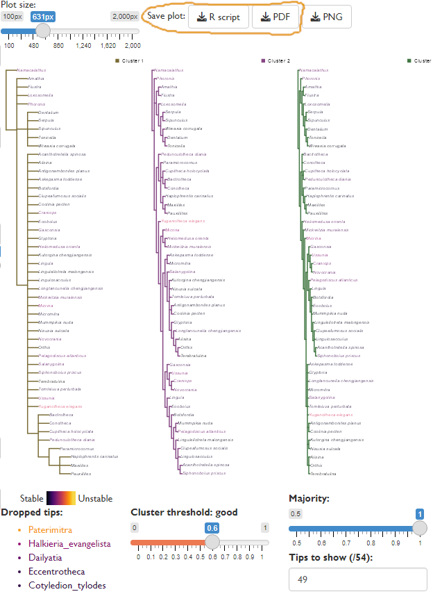
Plotting the consensus of trees within a specific cluster can give more insight into the underlying relationships within a tree set than viewing a single strict consensus, particularly where the data do not decisively distinguish between a small number of well-defined but conflicting phylogenetic hypotheses (Stockham et al., 2002).
Visualising the consensus of each cluster can reveal this “hidden” agreement between trees and allow more detailed and thoughtful analysis of the meaning of the phylogenetic output.
As the limited screen space available can render large trees difficult to read, it may be helpful to output the analysis using the “Save plot” options, either as an R script to allow further analysis within R, or as a PDF for more comfortable on-screen viewing.

The R code below is modified from that output by the GUI, in order to conduct rogue taxon analysis for each cluster separately. Note that it draws on the results of the clustering analysis above.
# Select proportion for majority rule consensus trees
# 1 is the appropriate value when parsimony trees are included
majority <- 1

# Plot each consensus tree in turn:
for (i in seq_len(nClusters)) {
  clusterTrees <- trees[clustering == i]
  # Identify rogue taxa for this cluster
  clusterRogues <- Rogue::QuickRogue(clusterTrees, p = majority)$taxon[-1]

  # Colour tree labels based on stability across cluster
  tipCols <- Rogue::ColByStability(clusterTrees)

  cons <- ConsensusWithout(
    trees = clusterTrees,
    tip = clusterRogues,
    p = majority
  )

  # Root tree
  cons <- RootTree(cons, trees[[1]]$tip.label[1])

  # Set unit edge lengths for viewing
  cons$edge.length <- rep.int(1, nrow(cons$edge))

  # Rotate nodes, to display clades in order of size
  cons <- SortTree(cons, order = names(trees[[1]]$tip.label))

  # Plot tree
  par(mar = c(0, 0, 0, 0), cex = 0.8) # Set up plotting area
  plot(
    cons,
    edge.width = 2,             # Widen lines
    font = 3,                   # Italicize labels
    cex = 0.83,                 # Shrink tip font size
    edge.color = clusterCol[i], # Colour tree according to previous plot
    tip.color = tipCols[cons$tip.label]
  )
  legend(
    "bottomright",
    paste("Cluster", i),
    pch = 15,            # Filled circle icon
    pt.cex = 1.5,        # Increase icon size
    col = clusterCol[i],
    bty = "n"            # Don't plot legend in box
  )
  if (length(clusterRogues)) {
    # Mark omitted taxa, if any rogues present
    legend(
      "topright",
      clusterRogues,
      col = tipCols[clusterRogues],
      text.col = tipCols[clusterRogues],
      pch = "-",      # Mark as excluded
      cex = 0.8,      # Smaller font
      text.font = 3,  # Italicize
      bty = "n"       # Don't plot legend in box
    )
  }
}
Where next?
-
Search for trees using
- standard parsimony (corrected for inapplicable data)
- profile parsimony
- custom optimality criteria