Information-based generalized Robinson–Foulds distances

Calculate tree similarity and distance measures based on the amount of phylogenetic or clustering information that two trees hold in common, as proposed in Smith (2020).

TreeDistance(tree1, tree2 = NULL)

SharedPhylogeneticInfo(
  tree1,
  tree2 = NULL,
  normalize = FALSE,
  reportMatching = FALSE,
  diag = TRUE
)

DifferentPhylogeneticInfo(
  tree1,
  tree2 = NULL,
  normalize = FALSE,
  reportMatching = FALSE
)

PhylogeneticInfoDistance(
  tree1,
  tree2 = NULL,
  normalize = FALSE,
  reportMatching = FALSE
)

ClusteringInfoDistance(
  tree1,
  tree2 = NULL,
  normalize = FALSE,
  reportMatching = FALSE
)

ExpectedVariation(tree1, tree2, samples = 10000)

MutualClusteringInfo(
  tree1,
  tree2 = NULL,
  normalize = FALSE,
  reportMatching = FALSE,
  diag = TRUE
)

SharedPhylogeneticInfoSplits(
  splits1,
  splits2,
  nTip = attr(splits1, "nTip"),
  reportMatching = FALSE
)

MutualClusteringInfoSplits(
  splits1,
  splits2,
  nTip = attr(splits1, "nTip"),
  reportMatching = FALSE
)

MatchingSplitInfo(
  tree1,
  tree2 = NULL,
  normalize = FALSE,
  reportMatching = FALSE,
  diag = TRUE
)

MatchingSplitInfoDistance(
  tree1,
  tree2 = NULL,
  normalize = FALSE,
  reportMatching = FALSE
)

MatchingSplitInfoSplits(
  splits1,
  splits2,
  nTip = attr(splits1, "nTip"),
  reportMatching = FALSE
)

Arguments

tree1, tree2

Trees of class phylo, with leaves labelled identically, or lists of such trees to undergo pairwise comparison. Where implemented, tree2 = NULL will compute distances between each pair of trees in the list tree1 using a fast algorithm based on Day (1985).

normalize

If a numeric value is provided, this will be used as a maximum value against which to rescale results. If TRUE, results will be rescaled against a maximum value calculated from the specified tree sizes and topology, as specified in the "Normalization" section below. If FALSE, results will not be rescaled.

reportMatching

Logical specifying whether to return the clade matchings as an attribute of the score.

diag

Logical specifying whether to return similarities along the diagonal, i.e. of each tree with itself. Applies only if tree2 is a list identical to tree1, or NULL.

samples

Integer specifying how many samplings to obtain; accuracy of estimate increases with sqrt(samples).

splits1, splits2

Logical matrices where each row corresponds to a leaf, either listed in the same order or bearing identical names (in any sequence), and each column corresponds to a split, such that each leaf is identified as a member of the ingroup (TRUE) or outgroup (FALSE) of the respective split.

nTip

(Optional) Integer specifying the number of leaves in each split.

Value

If reportMatching = FALSE, the functions return a numeric vector specifying the requested similarities or differences.

If reportMatching = TRUE, the functions additionally return an integer vector listing the index of the split in tree2 that is matched with each split in tree1 in the optimal matching. Unmatched splits are denoted NA. Use VisualizeMatching() to plot the optimal matching.

Details

Generalized Robinson–Foulds distances calculate tree similarity by finding an optimal matching that the similarity between a split on one tree and its pair on a second, considering all possible ways to pair splits between trees (including leaving a split unpaired).

The methods implemented here use the concepts of entropy and information (MacKay 2003) to assign a similarity score between each pair of splits.

The returned tree similarity measures state the amount of information, in bits, that the splits in two trees hold in common when they are optimally matched, following Smith (2020) . The complementary tree distance measures state how much information is different in the splits of two trees, under an optimal matching. Where trees contain different tips, tips present in one tree but not the other are removed before each comparison (as by definition, the trees neither hold information in common nor differ regarding these tips).

Concepts of information

The phylogenetic (Shannon) information content and entropy of a split are defined in a separate vignette.

Using the mutual (clustering) information (Meila 2007; Vinh et al. 2010) of two splits to quantify their similarity gives rise to the Mutual Clustering Information measure (MutualClusteringInfo(), MutualClusteringInfoSplits()); the entropy distance gives the Clustering Information Distance (ClusteringInfoDistance()). This approach is optimal in many regards, and is implemented with normalization in the convenience function TreeDistance().

Using the amount of phylogenetic information common to two splits to measure their similarity gives rise to the Shared Phylogenetic Information similarity measure (SharedPhylogeneticInfo(), SharedPhylogeneticInfoSplits()). The amount of information distinct to each of a pair of splits provides the complementary Different Phylogenetic Information distance metric (DifferentPhylogeneticInfo()).

The Matching Split Information measure (MatchingSplitInfo(), MatchingSplitInfoSplits()) defines the similarity between a pair of splits as the phylogenetic information content of the most informative split that is consistent with both input splits; MatchingSplitInfoDistance() is the corresponding measure of tree difference. (More information here.)

Conversion to distances

To convert similarity measures to distances, it is necessary to subtract the similarity score from a maximum value. In order to generate distance metrics, these functions subtract the similarity twice from the total information content (SPI, MSI) or entropy (MCI) of all the splits in both trees (Smith 2020) .

Normalization

If normalize = TRUE, then results will be rescaled such that distance ranges from zero to (in principle) one. The maximum distance is the sum of the information content or entropy of each split in each tree; the maximum similarity is half this value. (See Vinh et al. (2010, table 3) and Smith (2020) for alternative normalization possibilities.)

Note that a distance value of one (= similarity of zero) will seldom be achieved, as even the most different trees exhibit some similarity. It may thus be helpful to rescale the normalized value such that the expected distance between a random pair of trees equals one. This can be calculated with ExpectedVariation(); or see package 'TreeDistData' for a compilation of expected values under different metrics for trees with up to 200 leaves.

Alternatively, to scale against the information content or entropy of all splits in the most or least informative tree, use normalize = pmax or pmin respectively. To calculate the relative similarity against a reference tree that is known to be "correct", use normalize = SplitwiseInfo(trueTree) (SPI, MSI) or ClusteringEntropy(trueTree) (MCI).

References

MacKay DJC (2003). Information Theory, Inference, and Learning Algorithms. Cambridge University Press, Cambridge. https://www.inference.org.uk/itprnn/book.pdf.

Meila M (2007). “Comparing clusterings---an information based distance.” Journal of Multivariate Analysis, 98(5), 873--895. doi:10.1016/j.jmva.2006.11.013 .

Smith MR (2020). “Information theoretic Generalized Robinson-Foulds metrics for comparing phylogenetic trees.” Bioinformatics, 36(20), 5007--5013. doi:10.1093/bioinformatics/btaa614 .

Vinh NX, Epps J, Bailey J (2010). “Information theoretic measures for clusterings comparison: variants, properties, normalization and correction for chance.” Journal of Machine Learning Research, 11, 2837--2854. doi:10.1145/1553374.1553511 .

See also

Other tree distances: JaccardRobinsonFoulds(), KendallColijn(), MASTSize(), MatchingSplitDistance(), NNIDist(), NyeSimilarity(), PathDist(), Robinson-Foulds, SPRDist()

Author

Martin R. Smith (martin.smith@durham.ac.uk)

Examples

tree1 <- ape::read.tree(text="((((a, b), c), d), (e, (f, (g, h))));")
tree2 <- ape::read.tree(text="(((a, b), (c, d)), ((e, f), (g, h)));")
tree3 <- ape::read.tree(text="((((h, b), c), d), (e, (f, (g, a))));")

# Best possible score is obtained by matching a tree with itself
DifferentPhylogeneticInfo(tree1, tree1) # 0, by definition
#> [1] 0
SharedPhylogeneticInfo(tree1, tree1)
#> [1] 22.53747
SplitwiseInfo(tree1) # Maximum shared phylogenetic information
#> [1] 22.53747

# Best possible score is a function of tree shape; the splits within
# balanced trees are more independent and thus contain less information
SplitwiseInfo(tree2)
#> [1] 19.36755

# How similar are two trees?
SharedPhylogeneticInfo(tree1, tree2) # Amount of phylogenetic information in common
#> [1] 13.75284
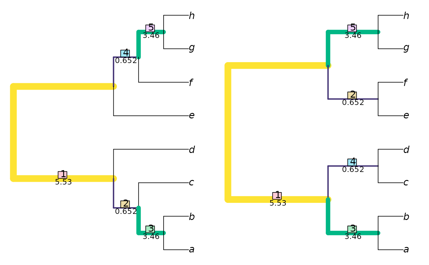
attr(SharedPhylogeneticInfo(tree1, tree2, reportMatching = TRUE), "matching")
#> [1] 1 4 2 3 5
VisualizeMatching(SharedPhylogeneticInfo, tree1, tree2) # Which clades are matched?


DifferentPhylogeneticInfo(tree1, tree2) # Distance measure
#> [1] 14.39934
DifferentPhylogeneticInfo(tree2, tree1) # The metric is symmetric
#> [1] 14.39934

# Are they more similar than two trees of this shape would be by chance?
ExpectedVariation(tree1, tree2, sample=12)["DifferentPhylogeneticInfo", "Estimate"]
#> [1] 31.25202

# Every split in tree1 conflicts with every split in tree3
# Pairs of conflicting splits contain clustering, but not phylogenetic, 
# information
SharedPhylogeneticInfo(tree1, tree3) # = 0
#> [1] 0
MutualClusteringInfo(tree1, tree3) # > 0
#> [1] 0.6539805

# Converting trees to Splits objects can speed up multiple comparisons
splits1 <- TreeTools::as.Splits(tree1)
splits2 <- TreeTools::as.Splits(tree2)

SharedPhylogeneticInfoSplits(splits1, splits2)
#> [1] 13.75284
MatchingSplitInfoSplits(splits1, splits2)
#> [1] 17.09254
MutualClusteringInfoSplits(splits1, splits2)
#> [1] 3.031424